Home page
QED is useless
Dirac equation is unreal
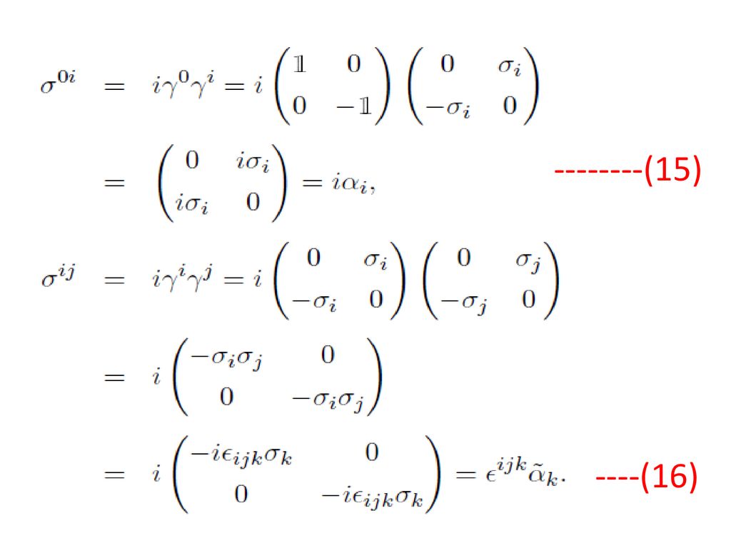
(Fig.1) Dirac equation expresses electron spin (= σμν ) as unphysical γ matrices .
Relativistic quantum field theory or QED relies on unphysical relativistic Dirac equation's γ matrices as (illusory) electron spin (= σμν = iγμγν, this-p.6-p.16 ).
↑ This relativistic Dirac equation's artificial spin has nothing to do with the real world's phenomena.
(Fig.2) ↓ unphysical artificial γ matrices = (illusory) spin ?
(Fig.3) relativistic metric tensor g
Using the unphysical γ matrices in relativistic Dirac equation, we get Fig.2 equation including the unphysical spin σμν 4 × 4 matrices.
This page uses (-1, +1, +1, +1) version of relativistic metric notation.
(Fig.4) artificial math trick of unphysical Dirac spin γ matrices.
(Fig.4')
By multiplying both sides of Fig.2 by pν u(p) and using Dirac equation, we get Fig.4 and Fig.4'.
About the notation, AνBν = A0B0 + A1B1 + A2B2 + A3B3 = -A0B0 + A1B1 + A2B2 + A3B3
(Fig.5) Artificial math trick-2 of Dirac unphysical γ matrices.
(Fig.5')
In the same way as Fig.4, we can get Fig.5 and Fig.5'.
(Fig.6)
By multiplying Fig.4' and Fig.5' by Fig.6- u or bar-u operator of Dirac equation, and summing them, we get Fig.7.
(Fig.7) Artificial math trick of linking Dirac γ matrices to magnetic moment, which is Not prediction by (useless) relativistic Dirac equation.
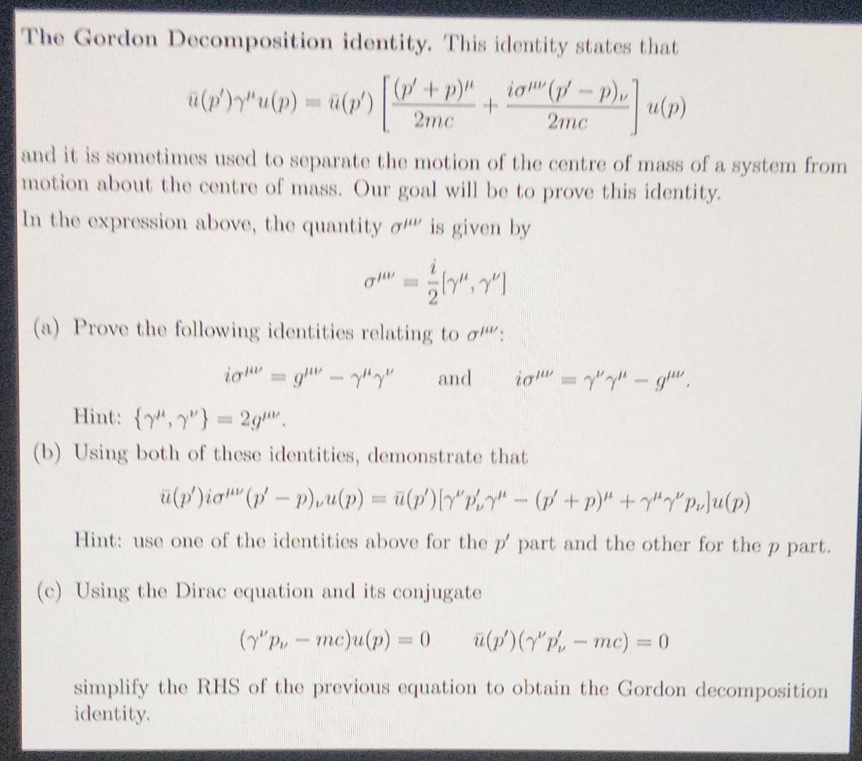
From Fig.4', Fig.5' and Fig.6, we obtain Fig.7 where the coefficient of the unphysical σμν is said to resemble the electron's magnetic moment (= Bohr magneton, this-p.2, this-p.12 ), which ad-hoc artificial process is called Gordon decomposition identity ( this-p.4, this-p.18, this-p.3-lower, this-p.12 ).
As shown here, the relativistic unphysical Dirac equation just artificially manipulating the unphysical γ matrices can Not predict the electron's magnetic moment or g-factor = 2, contrary to the standard explanation.
(Fig.8) ↓ Different inconsistent rules are applied to get Dirac spin g-factor (= 2 ) and QED anomalous magnetic moment (= g-2 ), which is Not prediction.
As shown in Fig.7 and Fig.8-artificial change-1, Dirac equation tries to artificially change the unphysical γ matrix into ( p' + p ) term (= momentum ? ) and σμν allegedly representing electron spin magnetic moment (= g = 2 ? this-p.8,p.10 ).
↑ This Dirac equation's derivation of electron spin g-factor or magnetic moment (= g= 2 ) is inconsistent with QED derivation of electron's smaller anomalous magnetic moment (= g-2 = 0.00116, this-p.13-14, this-p.3-p.4 ).
Because in QED calculation of electron anomalous magnetic moment, they use the different ad-hoc rule of artificially changing ( p' + p ) term into γ term (= illegitimately removed by renormalization ) and σμν (= this-artificial change-2 ), which is inconsistent with the above Dirac derivation of magnetic moment changing the γ matrix into ( p' + p ) term and the spin σμν term (= this-artificial change-1 ).
In Dirac's g = 2 factor in artificial change-1 of Fig.8, if they try to change ( p' + p ) term into other terms like anomalous magnetic moment of g-2 in artificial change-2, the spin term σμν (= allegedly expressing the original spin g-factor of g = 2 ) also disappears (= so this cannot get the electron's spin magnetic moment g = 2 ), and only γμ term remains. ← It means they get only Dirac g=2 factor or only the much smaller anomalous magnetic moment value of g - 2, if they try to apply the common change rule.
↑ Applying the inconsistent ad-hoc rules to Dirac's magnetic moment (= g = 2 ) and QED anomalous magnetic moment (= g - 2, this-p.3-(14)(17) ) means QED and relativistic Dirac equation are illegitimate, lacking power to predict any physical values such as anomalous magnetic moment.

Feel free to link to this site.