( xμ, pμ, and kμ = four-vectors )
Home page
QED is false
Quantum field theory.
On this web site, we use ( -1, +1, +1, +1) or (-+++) version of metric tensor.
So only the sign of the zero component of the four-vector changes by the index positions.
If you want to change to ( +1, -1, -1, -1 ) or (+---) version of metric tensor or signature, do as shown in Eq.1, Eq.2 and Fig.1-.
(Eq.1)
( xμ, pμ, and kμ = four-vectors )
And the matrices are
(Eq.2)
Basically, the meaning of the equations is completely the same in both ( -1, +1, +1, +1 ) and ( +1, -1, -1, -1 ) versions.
Only the notations are different in them.
So change only the signs ( + → -, or - → +) when encountering the letters with subindex like pμ → -pμ, and p2 (= pμpμ ) → -p2.
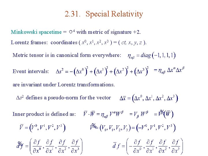
(Fig.1) time (= t or x0 ) and space (= xj or x,y,z ) variables
This website uses the metric signature of (-1,1,1,1) or (-+++) where only the sign of zero component vector (= time ) with subindex changes (= ct = x0 = -x0, where x0 = -ct ), while the space-component vectors do not change ( xj = xj, j = 1,2,3 ) their signs regardless of whether subindex or superscript in the spacetime four vectors ( this p.3, this p.3 ).
If you want to switch from (-1,1,1,1) or (-+++) into (1,-1-1-1) or (+---) version of metric signature, change the sign only of the space coordinate or 1-3 components ( xj = -xj j = 1,2,3 ) instead of the time variable or zero-component of four vectors.
(Fig.2) "c" is light speed.
Fig.2 is the relativistic energy (= E = cp0 ) and momentum (= p1, p2, p3 or px, py, pz ).
This website uses (-+++) version of 4-vector, tensor signature ( this-p.8, this-p.6, this-p.2-4 ).
If you want to switch from this website's (-1,+1,+1,+1) or (-+++) version of metric signature into (1,-1,-1,-1) or (+---) version, change only the sign of letters with subscript like pμ → - pμ
(Fig.3) Notation of relativistic energy (= E ) and momentum (= p )
Using Fig.2, relativistic energy-momentum-mass relation is expressed like Fig.3.
In this notation rule, when the same letter is used twice in one term like pμpμ or p2, it means the sum of all μ = 0,1,2,3 components (= even when the summation simbol Σ is not added ) like the upper figure ( this p.9, this p.3-4, this p.2 ).
(Fig.4)
In the derivative (= ∇ or ∂ ) or differential operators, when the index is at the lower position (= subindex or subscript ), it means the common normal differential operator.
When the index position is at the higher position (= superscript ), the sign of only the zero component (= time ) differential operator switches into the negative, while the signs of all other space derivatives remain the same irrespective of the index position in this website (-1,1,1,1) version of metric signature.
In the (1,-1-1-1) version of metric signature, the sign of the differential operator with superscript becomes the opposite where only space differential operators become negative, while the sign of the zero-component time differential operator does not change irrespective of the index position ( this p.2 ).
(Fig.5)
(Fig.6)
Relativistic energy (= E = ℏω where ω is relativistic fictitious angular frequency, ℏ = h/2π where h is Planck constant ) and momentum (= p ) can be expressed as differential operators together with the exponential function of the relativistic wavefunctions ( this p.2 ), based on de Broglie wavelength theory.
Here we use "four-vector potential (= this vector potential is an invisible fictitious potential introduced only for nonphysical theoretical calculations )" like current density, as follows,
(Fig.7)
In Fig.7, "A" is vector (magnetic) potential allegedly used for expressing the magnetic field B, and "φ" is scalar (electric) potential allegedly used for expressing the electric field E.
(Fig.8) On this website (-1,1,1,1), only the zero-component changes its sign in its subindex.
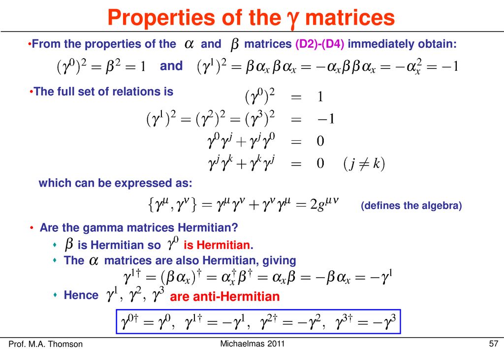
Relativistic Dirac equation uses nonphysical γ matrices like
(Fig.9)
where I means 2 × 2 identity matrix.
(Fig.10)
γ0γ0 = I ( = 4× 4, identity matrix ),
(Fig.12)
(Fig.14)
(Fig.15)
(Fig.16)
Using Fig.2 and Fig.4,
the relativistic Dirac equation can be expressed like Fig.16.
(+1,-1,-1,-1) version of Dirac equation is in this p.20, this p.2-3.
This website uses (-1, +1, +1, +1) version of notation.
(Fig.17)
Using the metric tensor (= gμν ), the relativistic momentum and energy can be expressed like Fig.17.
Here we calculate and prove the conversion of the QED anomalous magnetic moment's equations in Fig.6 of this page.
(Eq.3) QED artificial math trick in calculating anomalous magnetic moment.
(Eq.4) k' = virtual electron-2, k = virtual electron-1, q is a photon's energy and momentum.
In the unphysical QED electron's anomalous magnetic moment's one loop correction, the sum of energy and momentum of the virtual electron-1 (= k ) and a photon (= q ) becomes the virtual-electron-2 (= k' ).
This page uses the relativistic 4-vector notation of (-1,1,1,1).
(Eq.5) QED illegitimate change of variables adds new zp values to the numerator as an artificial magnetic moment.
After QED's illegitimate change of variables ( l = k + yq - zp where l and k represent unrealistic virtual particles' energies from - infinity to + infinity ), new values such as yq - zp artificially appear in the numerator, which are used as a part of the artificial anomalous magnetic moment.
They ignore and eliminate all terms linear to this l (= zero, as shown in Eq.5-lower ) by integration from -∞ to +∞ ( this p.3-3rd-paragraph ), because change of variables by finite values ( l = k + yq - zp ) does not change the upper (= + infinity ) and lower (= - infinity ) numbers of variables k and l, which is one of QED tricks ( this-p.54-(5.20)-(5.24), this-p.146 ).
This is one of QED illegitimate tricks artificially manipulating physical values, combined with the renormalization removing infinities.
(Eq.6) QED anomalous magnetic moment's calculation uses this artificial math formula ↓
(Eq.6') QED Dirac equation formula
The calculation of QED anomalous magnetic moment uses the math formula of Eq.6 where p is relativistic energy (= p0. p'0. q0 ) and momentum (= pa, p'a, qa, a = 1, 2, 3 ), γ is unphysical matrices, and relativistic Dirac equation ( here approximately, c = ℏ = 1 ).
See this-p.2-middle, this-p.146-147, this-p.25(or p.22)-last, this-p.17
(Eq.7) QED artificial calculation-2 of electron's anomalous magnetic moment.
Here we explain the detail calculation of Fig.7 converting Eq.A to Eq.B of artificial QED anomalous magnetic moment.
Using this QED formula, we have
(Eq.8)
where the sum of the momentum and energy of electron-1 (= p ) and a photon (= q ) becomes the electron-2 (= p' )
Using this formula, we have terms of ①, ②, ③ in Eq.8-lower equation, as follows,
(Eq.9)
(Eq.10)
(Eq.11)
where we use the relativistic mass formula.
Summing Eq.8, terms of ① ~ ⑤ including Eq.9, Eq.10, Eq.11, we can get the conversion from Eq.A to Eq.B, as follows,
(Eq.12) artificial QED conversion from Eq.A to Eq.B
where we use p' = p + q.
Using various illegitimate math tricks, QED managed to get (artificial) anomalous magnetic moment value ( this-p.1-right, this-p.13-18, thid-p.52(p.46)-p.59 ).
This section is moved from Eq.4-7 (Eq.4-4) to Eq.4-11 of this page.
(Eq.4-4)
For example, when we calculate the next propagator, which means the transmission of the particle,
(Eq.4-7)
where Eq.4-19 is used.
(Eq.4-19)
Two square roots of ω in Eq.4-4 change to
(Eq.4-8)
After integrating with respect to one d3k , so only another k is left here.
We use the following formula in delta function.
(Eq.4-9)
Taking the formula of Eq.4-9, we can get
(Eq.4-10)
where we use Eq.4-1.
(Eq.4-1)
Adding d4p to Eq.4-10, and integrating Eq.4-10 with respect to p0, we get the equation of
(Eq.4-11)
where θ means "step function".
Eq.4-11 contains the integration of d4p and Eq.4-1, so this is Lorentz invariant.
( Of course, integral region must be from minus infinity to plus infinity to make d4p Lorentz invariant. )
So Eq.4-8 is Lorentz-invariant, too.
As you notice, we can change the coefficients such as c and h freely, keeping Lorentz invariance.
So we can adjust these values "artificially" to get the correct energy values.
Feel free to link to this site.