Home page (11/2025)
Topological quantum computer is illusion
Topological insulator is useless.
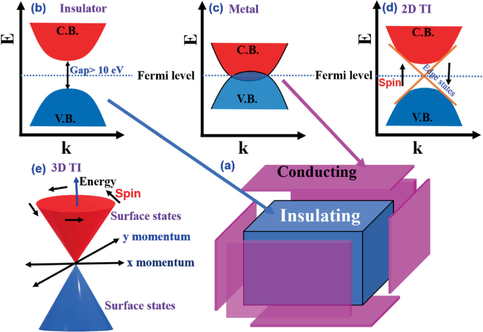
(Fig.1) Topological insulator just shows some electric conductance at very low tempeture = energy-inefficient, impractical.
Topological insulator (= TI ) is useless material whose edge (= in 2-dimensional TI ) or surface (= in 3-dimensional TI ) is conductive, and the remaining bulk part is insulator.
Overhyped media tend to baselessly tout this topological insulator as dreamlike material with lossless energy or no energy dissipation, which promises to be an energy-efficient device ( but actually, topological insulator remains useless, stuck in the ambiguous hyped "promising" stage forever ).
This-p.2-last-paragraph says -- Topological energy dissipation
"we discovered
notable energy dissipation inside the topological devices which are typically referred as
dissipationless"
The 1st, 7-8th paragraphs of this or this recent site say
"Topological insulators are promising materials for application in electronics because they efficiently conduct electricity, reducing energy consumption... Their application in consumer products is very challenging though, since they only function at very low temperatures (= topological insulator is still useless )."
"But in topological insulators, electricity flow is unaffected by impurities and consequently, there are no energy losses (= No evidence )... However, they are not applied in consumer products yet, because they are difficult to make and can only operate at very low temperatures (= still impractical topological insulator )."
"Science on these special insulators is still in the very fundamental phase. ‘Although use in consumer products is still a long way off, "
↑ This kind of media narrative is self-contradictory, because topological insulator, which can be operated only at very low temperature, is clearly useless and energy-inefficient (= wasting a lot of energy to keep the extremely-low temperature ).
The 1st and 3rd paragraphs of this recent news also say
"However, topological insulators fail to maintain this lossless 'magic' at room temperature."
"topological insulators face serious challenges in maintaining their feature in a practical working environment," ← topological insulator is still impractical (forever).
This review's p.5-2nd-paragraph says -- Useless topological insulator
"Topological insulators present unique opportunities for device applications, but realizing useful
topological devices remains challenging."
The 5th-paragraph of this hyped news about the alleged zero energy loss topological insulator also admits
"There was just one problem: these properties were discovered only in.. very low temperatures, around minus 270 degrees Celsius, which made them not suitable for use in daily life."
↑ This research paper (p.2-last-paragraph ~ p.3-Fig.1) just measured finite electric conductance (= dI/dV = Not zero resistance means this topological insulator's current loses energy ) of the topological insulator at impractically-low temperature 4K, which is useless, energy-inefficient, and far from zero-energy-loss.
This p.9-~p.12 say the topological insulator containing two electric currents with up and down (imaginary) spins flowing in the opposite directions should show some electric conductance 2e2/h or resistance of 2h/e2 (= which is called quantum spin Hall effect used as evidence of topological insulator, but the electron spin itself is unreal, undetectable in topological insulator ).
↑ This research paper about the the first discovery of topological insulator ( this p.26 ) ↓
p.4-2nd-paragraph says "massless Dirac model (= fictional quasiparticle ) with M = 0,... to a negative value M < 0 (= unreal negative mass ) for thick quantum wells"
p.9-last ~ p.10 mentions "Clearly, in this further sample, and at 1.8K, the 2e2/h conductance plateau is again present (= 1.8K is too low temperature to be practical )"
p.9-1st-paragraph says "reaches the predicted value close to 2e2/h. This observation provides firm evidence for the existence of the quantum spin Hall insulator state (p.20-Fig.4)"
↑ This research just vaguely measured electric conductance 2e2/h (= 1/resistance, this p.12 ) at extremely low temperature ( this p.3-Fig.2, prediction and discovery ), and did Not measure the electron spin itself, lossless energy nor fictional massless quasiparticle, so No evidence of topological insulator nor quasiparticle's (pseudo-)spin.
(Fig.2) An electron with real mass ejected by incident light in ARPES must be intentionally misinterpreted as a (fictional) Dirac quasiparticle with fake effective mass in topological insulator.
The reason for the (baseless) lossless energy of the topological insulator depends on the unphysical (= mathematical ) topologically-protected time reversal symmetry ( this or this p.4-p.5 ), which has No real evidence.
Physicists often use ARPES (= Angle-Resolved photo emission spectroscopy ) to measure the kinetic energy and momentum of an electron (= with real mass ) ejected by incident light, and wrongly infer the (imaginary) momentum (and energy) of a fictional massless Dirac fermion quasiparticle ( this 2nd-paragraph, this p.2-Fig.1, p.2-right, this p.4-right ) inside topological insulator.
↑ This ARPES detecting only the vague scattering direction of a real electron with real mass cannot directly measure the (fictional) electron spin and quasiparticle with fake effective mass.
This discrepancy in (mis-)interpretation of ARPES measurement results is caused by using freely-adjustable parameter V0 called inner potential to wrongly guess fake effective mass (= like massless ) of a fictional quasiparticle (= imaginary theory ) from the measurement of the momentum and energy of a real electron with real mass ejected by light ( this p.1-abstract, this p.32, this p.12 ).
Furthermore, they baselessly concluded that (fictional) quasiparticle electrons with up and down spins on the edge or surface of the topological insulator have the opposite quasi-momentum, which is preserved or topologically-protected due to (unphysical) time-reversal symmetry ( this p.20, this 2nd~3rd-paragraphs, this p.13-p.16 ), which topological protection has No evidence.
This research (p.2) also baselessly concluded that some material was a topological insulator with fictional Dirac quasiparticle protected by (unphysical) time reversal symmetry, after measuring only (photo-)electrons ejected by light in ARPES ( this p.26-27,p.33, this p.4-6 ).
As a result, the overhyped topological insulator is useless with No evidence of lossless energy due to (imaginary) topological protection based on mathematical time reversal symmetry or fictional Dirac quasiparticle with pseudo-spin.
The 1st, 7th paragraphs of this overhyped news (6/23/2025) say
"A team.. has made a breakthrough in the development of ultra-thin magnets—a discovery that could (= just speculation, still useless ) lead to faster, more energy-efficient electronics, quantum computers, and advanced communication system" ← hype
"The ultra-thin magnet alone worked at around 100 Kelvin, but when combined with the topological insulator, its strength further improved by 20%, functioning at higher temperatures (cf. liquid nitrogen 77 Kelvin)." ← impractically-low temperature, energy-inefficient.
↑ This research paper's p.3-abstract says nothing about "faster, energy-efficient quantum computers", contrary to the above overhyped fake news

Feel free to link to this site.